Cost Design in Atomic Routing Games
03 Oct 2022 | publication
Yue Yu,
Shenghui Chen, David Fridovich-Keil,and Ufuk Topcu
American Control Conference, 2023
Motivation
Transportation is crucial in our daily lives. Picture an intersection with four cars, each wanting to reach the opposite side of the road. The instinctive choice for each car would be the shortest path, directly crossing the intersection. However, this would lead to congestion at the center of the intersection. What’s a better solution for a socially optimal interaction? In reality, a roundabout is often implemented as an alternative. It slows down vehicles and enhances transportation efficiency by requiring each car to take a slightly longer route. (See comparison in the animation below.)
| Before Design |
After Design |
 |
 |
In this paper, we study the problem of designing the right cost structure that encourages players to choose the roundabout—a more desirable social interaction—instead of direct crossings.
Atomic Routing Games
Routing games are the fundamental mathematical models for predicting the collective behavior of selfish players in transportation networks. A routing game is a multi-player game on a directed graph.
A directed graph \(\mathcal{G}\) contains a set of nodes \([n]\) and a set of directed links \([m]\) where each link is an ordered pair of “tail” node to “head” node. We characterize the connection among nodes in the graph \(\mathcal{G}\) by the incidence matrix \(E\in\mathbb{R}^{n\times m}\) where
$$
\begin{align}
\left[E\right]_{ij}=\begin{cases} 1, & \text{if node i is the tail of link j,}\\
-1, & \text{if node i is the head of link j,}\\
0, & \text{otherwise.}
\end{cases}
\tag{1}
\end{align}
$$
On a directed graph characterized by \(E\), an atomic routing game considers \(p\in\mathbb{N}\) players where each player \(i\in[p]\) has an origin node \(o_i\in[n]\) and a destination node \(d_i\in[n]\) in graph \(\mathcal{G}\). Let \(r_i\in\mathbb{R}^n\) denote the the origin-destination vector of player \(i\) such that
$$
\begin{align}
\left[r_i\right]_{j}=\begin{cases} 1, & \text{if } j = o_i,\\
-1, & \text{if } j = d_i,\\
0, & \text{otherwise.}
\end{cases}
\tag{2}
\end{align}
$$
Then let \(s_i=\Gamma(r_i, d_i)\in\mathbb{R}^{n-1}\) denote the reduced origin-destination vector obtained by deleting the \(d_i\)-th element in \(r_i\). We also define the notion of reduced incidence matrix for player \(i\) by \(E_i:=\Gamma(E, d_i)\). Hence, we define the feasible flow set for player \(i\) by \(\mathbb{P}_i\subset \mathbb{R}^m\) as
$$\mathbb{P}_i=\{y\in\mathbb{R}^m | E_i y=s_i,\, y\ge 0\}, \quad \forall i\in[p]. \tag{3}$$
Each player \(i\in[p]\) chooses a path from its origin node \(o_i\) to its destination node \(d_i\). We represent the path chosen by player \(i\) via a flow vector \(x_i\in\mathbb{R}^m\), where \([x_i]_k\in [0,1]\) denotes the probability for player \(i\) to use link \(k\) on the chosen path. By the definition above, if vector \(x_i\) is a valid path connecting nodes \(o_i\) and \(d_i\), then it belongs to a feasible flow set. In other words, \(x_i\in\mathbb{P}_i\) if and only if \(x_i\) is a unit flow that originates at node \(o_i\), ends at node \(d_i\), and is preserved at any other node.
Forward Game Solution
We assume the cost of each player \(i\in[p]\) is in the form of
$$
\begin{align}
b_i + \frac{1}{2}C_{ii}y + \sum_{j\ne i} C_{ij} x_j,
\tag{4}
\end{align}
$$
where \(b_i\in\mathbb{R}^m\) is the nominal link cost independent of the players’ choices, and \(C_{ij}\in\mathbb{R}^{m\times m}\) for all \(i,j\in[p]\) are matrices of cost adjustments introduced due to interactions with other players.
We introduce the notion of Nash equilibrium in an atomic routing game as a joint flow \(x:=\begin{bmatrix} x_i^\top \dots x_p^\top\end{bmatrix}\) where \(\forall i\in[p]\),
$$
\begin{align}
x_i \in \arg\min_{y\in \mathbb{P}_i} \quad & \left(b_i + \frac{1}{2}C_{ii}y + \sum_{j\ne i} C_{ij} x_j\right)^\top y.
\tag{5}
\end{align}
$$
In the paper, we show how to compute this Nash equilibrium by solving a set of piecewise linear equations. However, since the nonsmooth piecewise linear equations are difficult to solve in general, we propose an approximate solution with smooth nonlinear equations instead. To this end, we first introduce an entropy-regularized Nash equilibrium below as an apprximation solution concept.
Forward Game Solution: Entropy-regularized Nash equilibrium
A joint flow \(x:=\begin{bmatrix} x_i^\top \dots x_p^\top\end{bmatrix}\) is an approximate Nash equilibrium if all players \(i\in[p]\) choose flow vectors \(x_i\) as follows:
$$
\forall i \in [p] \quad \begin{cases}
\begin{align}
\min_{x_i} \quad & \left(b_i + \frac{1}{2}C_{ii}x_i + \sum_{j\ne i} C_{ij} x_j\right)^\top x_i + \lambda x_i^\top \ln(x_i)\\
\text{s.t.} \quad & E_i x_i = s_i\\
\quad & x_i\ge 0\\
\end{align}
\end{cases}
\tag{6}
$$
where \(\lambda\in \mathbb{R}_{\ge 0}\) is an entropy weight.
This problem can be approximately solved by converting to a nonlinear least-squares problem (see detailed derivation in Lemma 2 of our paper):
Forward Game Solution: Nonlinear Least Squares
\(x,v=\textbf{Ent-NE}(b,C)\) iff \(x,v\) solves the nonlinear least squares problem
$$\begin{align}
\min_{x, v} \quad &\left\|x-\exp\left(\frac{1}{\lambda}(E_{[1,p]}^\top v - b - Cx) - \mathbf{1}_{pm}\right)\right\|^2 \\
&+ \left\|E_{[1,p]}x-s\right\|^2
\end{align}
\tag{7: Ent-NE}
\label{Ent-NE}$$
We assume the matrix \(C\) bears a specific structure that can ensure the uniqueness of the solution (see Assumption 1 and Theorem 1 in our paper).
Inverse Cost Design
We now introduce the cost design problem in atomic routing games. The task is to design the value of a vector \(b\) and a matrix \(C\) such that the entropy-regularized Nash equilibrium \(x\) optimizes certain performance function \(\psi(x)\),
$$
\begin{align}
\min_{x,v,b,C} \quad &\psi(x) = \frac{1}{2} \|x-\hat{x}\|^2\\
\text{s.t.} \quad &x,v = \textbf{Ent-NE}(b,C)\\
\quad &b\in\mathbb{B}, C\in\mathbb{C}
\tag{8}.
\end{align}
$$
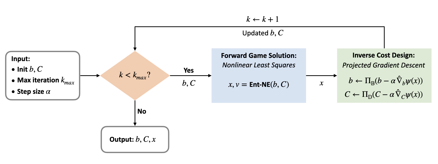
To solve this problem, we propose an algorithm that iteratively
- Forward game solution: solves an equilibrium \(x\) with the current cost parameters \(b,C\) using \ref{Ent-NE}.
- Inverse cost design: updates \(b, C\) by projected gradient descent until the solution converges to a desired equilibrium \(\hat{x}\) or reaches the maximum number of iterations.
The key step in inverse cost design is to differentiate through the approximate Nash equilibrium conditions.
Inverse Cost Design: Implicit Differentiation
We focus on the derivation of \(\nabla_b\psi(x)\); similar logic applies to \(\nabla_C\psi(x)\).
$$
\begin{align}
\nabla_b\psi(x) &= \partial_b x^\top \cdot \nabla_x \psi(x) = \partial_b \begin{bmatrix}x^\top v^\top\end{bmatrix}^\top \cdot \begin{bmatrix}\nabla_x \psi(x) \\ 0_{p(n-1)}\end{bmatrix}
\tag{9}
\end{align}
$$
Let \(\xi = \begin{bmatrix}x^\top v^\top\end{bmatrix}^\top\), we need to compute \(\partial_b\xi\) and \(\nabla_x\psi(x)\). The latter is straight-forward to compute since \(\psi(x)\) only depends on \(x\). To derive the former, we first let
$$
F(\xi, b, C) := \begin{bmatrix}x-\exp\left(\frac{1}{\lambda}(E_{[1,p]}^\top v - b - Cx) - \mathbf{1}_{pm}\right) \\ s-E_{[1,p]}x \end{bmatrix},
\tag{10}
$$
and by the
implicit function theorem, we have if \(\partial_\xi F(\xi, b, C)\) is nonsingular, then
$$
\partial_b \xi = -\left(\partial_\xi F(\xi, b, C)\right)^{-1}\partial_b F(\xi, b, C)
\tag{11}
$$
which can be done since \(\xi\) and \(b\) are variables of the function \(F\).
We adopt \(\hat{\nabla}_b\psi(x)\) in practice, where we use the Moore-Penrose pseudoinverse of a matrix whose inverse may not exist. Check Theorem 2 in
our paper for more details.
After a step of gradient descent, we project the new cost parameters to defined spaces in order to satisfy the uniqueness assumption posed.
Inverse Cost Design: Projections
The projection maps \(\Pi_{\mathbb{B}}:\mathbb{R}^m\to \mathbb{R}^m\) and \(\Pi_{\mathbb{D}}:\mathbb{R}^{m\times m}\to \mathbb{R}^{m\times m}\) are given by
$$
\begin{align}
\Pi_{\mathbb{B}}(b) &= \arg\min_{z\in\mathbb{B}}\|z-b\|,\\
\Pi_{\mathbb{D}}(C) &=\arg\min_{X\in\mathbb{D}}\|X-C\|_F,
\tag{12}
\end{align}
$$
and we choose spaces
$$
\begin{align}
\mathbb{B}:=\{&b\in\mathbb{R}^{pm}|0_{pm}\le b\le \delta\mathbf{1}_{pm}\},\\
\mathbb{D}:=\{&C\in\mathbb{R}^{pm\times pm} | C+C^\top\succeq 0,\, \|C\|_F \leq \rho,\, C_{ii}=C_{ii}^\top,\; \forall i\in[p]\},
\tag{13}
\end{align}
$$
where parameters \(\delta\) and \(\rho\) control the amount of variation allowed for \(b\) and \(C\), respectively.
Numerical Result

Implementation Note
We implemented the algorithms in Julia using the JuMP interface. The nonlinear optimization in the \ref{Ent-NE} is solved by IPOPT. In this work, we hand-derived all the gradients, but they can also be easily computed with the auto-grad tools, e.g., Zygote. Check out our code on github for more details.