A function primer for optimization
30 Dec 2022 | learning notes- 1. Continuous
- 2. Differentiable
- 3. \(k^{th}\) Continuously Differentiable and Smooth
- 4. Convex vs Nonconvex
- 5. Linear vs Nonlinear
- References
1. Continuous
Intuitively, a function is continuous if its graph is a single unbroken curve (in two-dimension).
A discontinuous function, instead, is not continuous and has gaps in its graph, known as discontinuities. These gaps include holes, jumps, and asymptotes.
Formally, we can define continuity using epsilon-delta limit:
A function \(f\) is continuous when, for every value \(c\) in its domain, \(f(c)\) is defined, and \(\lim_{x\to c} = f(c)\).
2. Differentiable
A function is differentiable means its derivative exists for every value in its domain.
Formally, the derivative for a function \(\phi: \mathbb{R} \to \mathbb{R}\) is defined as
\[\phi'(\alpha) = \lim_{\epsilon\to 0}\frac{\phi(\alpha +\epsilon)-\phi(\alpha)}{\epsilon}\]Similarly, the second derivative is obtained by susituting \(\phi\) by \(\phi'\), i.e.,
\[\phi''(\alpha) = \lim_{\epsilon\to 0}\frac{\phi'(\alpha +\epsilon)-\phi'(\alpha)}{\epsilon}\]Differentiability has intimite relationship with continuity:
\[\text{Differentiable} \quad \Rightarrow \quad \text{Continuous}\]This means a differentiable function is necessarily continuous, but a continuous function may not be differentiable. For example, \(f(x)=\lvert x \rvert\) is continuous (no gaps) but not differentiable since derivative does not exists at \(x=0\) (pointy turn).
Now consider the function \(f:\mathbb{R}^n\to \mathbb{R}\), with variables usually gathered as \(x=(x_1, x_2, \dots,x_n)^T\). We say \(f\) is differentiable at \(x\) if there exists a vector \(g\in\mathbb{R}^n\) such that
\[\lim_{y\to 0}\frac{f(x+y)-f(x)-g^Ty}{\|y\|}=0\]We call such \(g\) the gradient of \(f\) at \(x\) and denote it by \(\nabla f(x) = [ \frac{\partial f}{\partial x_1} \dots \frac{\partial f}{\partial x_n}]^T\).
3. \(k^{th}\) Continuously Differentiable and Smooth
We say a function \(f\) is continuously differentiable if \(\nabla f(x)\) is a continuous function of \(x\).
Similarly, \(f\) is twice continuously differentiable on its domain \(\mathcal{D}\) if \(\nabla^2 f(x)\) exists for all \(x\in\mathcal{D}\) and is continuous on \(\mathcal{D}\).
By this logic, we can have \(k^{th}\) continuously differentiable function if \(\nabla^k f(x)\)exists for all points in its domain, for some \(k\in \mathbb{N}\).
According to wikipedia,
the smoothness of a function is a property measured by the number of continuous derivatives it has over some domain.
-
At the minimum, a function can be called smooth if it is differentiable;
-
Some smooth functions is finitely-times differentiable (\(k^{th}\) differentiable);
-
At the other end, a function can be infinitely differentiable, that is, it possesses derivatives of all orders in its domain.
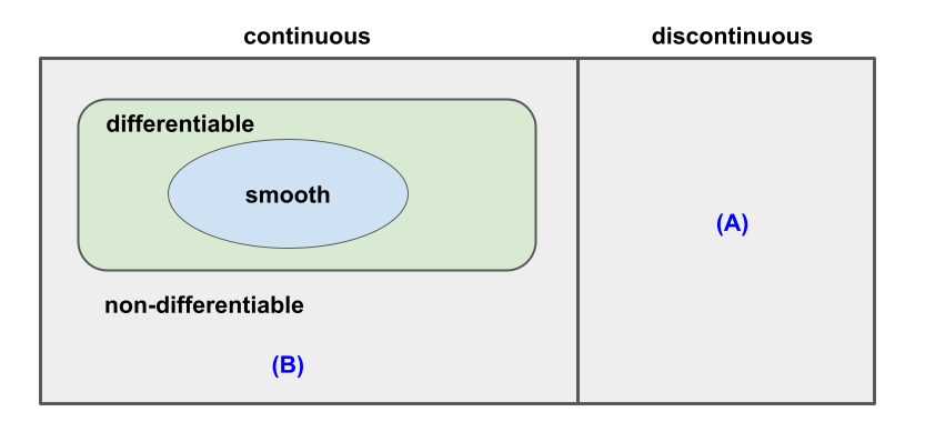
In summary, we can arrive at a venn-like relationship diagram below:

There is a discipline called nonsmooth optimization, as opposed to optimization that focused on smooth functions, there
- (A) It is not possible in general to identify a minimizer of a general discontinuous function;
- (B) If the function is continuous everywhere but nondifferentiable at certain points, we can identify a solution by examing the subgradient or generalized gradient;
- If the function consists of a few smooth pieces with discontinuities in between, we can solve by minimizing each smooth piece individually (converting the problem to a series of smooth optimization problems).
4. Convex vs Nonconvex
- Convex Set: A set \(S\in\mathbb{R}^n\) where the straight line connecting any two points in \(S\) lies entirely in \(S\), \(\forall x, y\in S\),
- Convex Function: A function \(f\) whose domain \(S\) is a convex set and \(\forall x, y\in S\),
- An important result in optimization states that if the objective function and the feasible region in a problem are both convex, then any local solution of the problem is a global one. However, if a problem is non-convex, then there may be more than one feasible region and we cannot guarantee a local optimal solution in one region is indeed the globally optimal. That means, convex problems are intrinsically easier to solve than non-convex problems.
5. Linear vs Nonlinear
Linear functions form straight lines when plotted; while nonlinear functions from lines that are curved in some way.
For an optimization problem, if it has a linear objective function, subject to linear constraints, then we can use Linear Programming (LP) to solve it.
Linear programs are problems expressed in canonical form below:
\[\begin{align*} \min_x \quad &c^T x\\ \text{s.t.} \quad &Ax= b\\ \quad &x\ge 0 \end{align*}\]For a linear program, its feasible region is a convex polytope, and the objective function is an affine function defined on this polytope.
The difference between linear and nonlinear problems in optimization mainly stems from their convexity as explained in previous section. Since all linear functions are convex, LP problems are also intrinsically easier to solve than general nonlinear problems, which may be non-convex.
References
- Wright, Stephen, and Jorge Nocedal. “Numerical optimization.” (1999).
- “Continuous Functions.” Math Is Fun Advanced.
- “Differentiable”. Math Is Fun Advanced.
- “Smoothness”. Wikipedia.